2. Dynamic Matrix Control
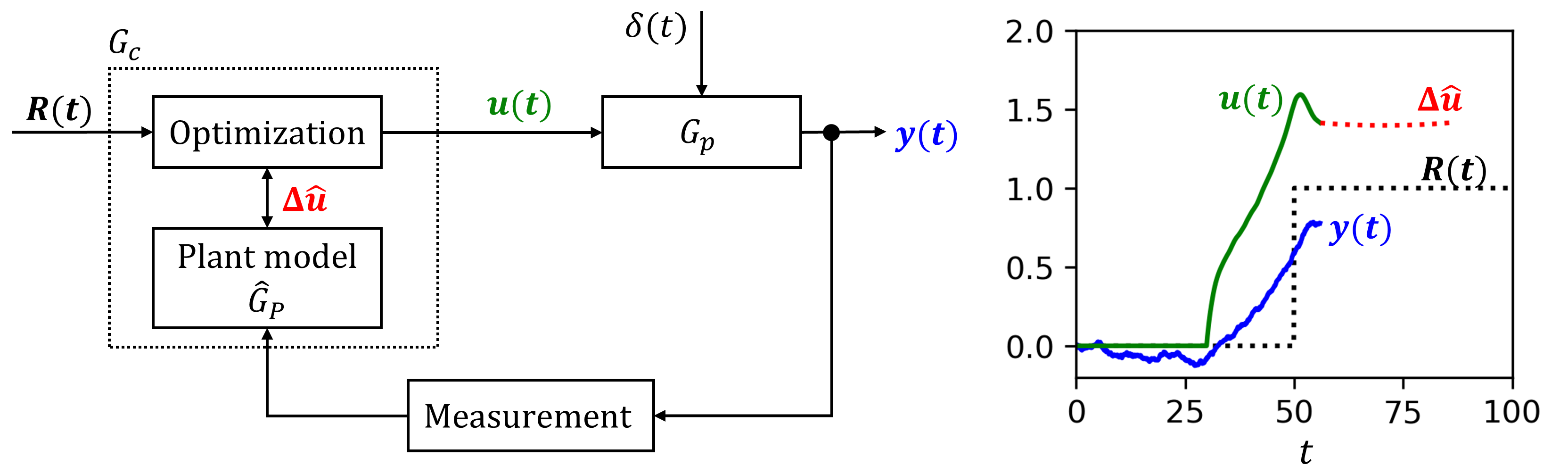
Written on June, 2025 by Bolton TranDynamic Matrix Control (DMC) is one of many methods under a class called Model Predictive Control (MPC). These methods use an approximate model of the plant/process $\hat G_p$ to guess a change in manipulated variable $\Delta\hat u$, and iteratively optimize it to minimize the process variable deviation from the setpoint ($y(t)$$- R(t)$) as well as the magnitude of change in manipulated variable $u(t)$.
Introduction and theories
Consider a first-order plant/process, we can write the ODE:
The variables are similar to those in Part 1. PID controller, but rewritten in the symbols of state-space convention, i.e., $y:=C; u:=M$. We also assume a unit process gain $K_p$, i.e., the controller output $u$ scale 1:1 with the process output $y$. $\tau$ is the process time constant. $\delta(t)$ is simply a fluctuating load following some normal distribution, added to simulate real process noise.
Previously with PID controller, $u(t)$ defines and constructs the controller block. Here, with DMC, an approximate plant/process model $\hat G_p$ is firstly required:
Note that $\hat G_p$ is not the same as the $G_p$ in Eqn. 1, which is the hypothetically “real-life” plant process. Say we performed experiments and determined the first-order dynamics and the time constant $\tau$ of this real-life process. Say we know not the form of load fluctuation $\delta(t)$, so it has been removed in the approximate model we constructed.
Furthermore, we know the exact analytical form of $u(t)$ for the PID controller, but now we do not. With DMC, we instead dynamically update $u(t)$ at each time step by using an optimization procedure. The optimization goes hand-in-hand with the approximate plant model $\hat G_p$, which collectively define the DMC controller block (see above diagram).
Real-life plant
Again, we do not have a physical plant to obtain process variable from, so we solve a model and call it “real-life.” As before, we iterate through discrete time steps and solve the controller logic. At time step $k$, we use the finite difference approximation to forward-predict the next $y_{k+1}$ from the real plant model $G_p$.
For simplicity, we wrote $\left(1-\frac{\Delta t}{\tau} \right)=A$ and $\frac{\Delta t}{\tau}=B$.
DMC logics
The crux of the DMC controller is a horizon prediction window $N$. At any given time $t=k$, the approximate plant model $\hat G_p$ will make prediction for $N$ steps into the future, i.e., at $t=k+1; k+2,…,k+N$.
Mimicking the form of the real plant (Eqn. 3), $\hat G_p$ predicts the output at the next multiple time steps that fall inside the horizon $N$ as follows.
Each subsequent iteration from $k+1$ to $k+N$ depends on the previous step, leading to this patterned series of summation (working out these equations on paper is helpful). That hats on $\hat y_{k+1}$ and $\hat u_k$ indicate that these come from the approximate model $\hat G_p$. No hat is on the initial $y_k$, which comes from the real plant’s output (Eqn. 3).
We next write Eqn. 4 in matrix form.
Rewrite in algebraic form (bold symbols are matrices):
The subscript $\mathbf{k}$ on $\mathbf{\hat y_k}$ and $\mathbf{\hat u_k}$ reminds us that this equation applies to some given time step $k$, though the elements inside those matrices contain predictions to future time steps.
Finally, we break the predicted manipulated variables $\mathbf{\hat u_k}$ at time $k$ into that at time $k-1$ plus a step-change term.
The reason for doing this will be clearer when we look at the optimization procedure.
DMC optimization
We saw that each time $k$, we are making a series of prediciton for process variable $y$ for $N$ steps into the future by using a series of manipulated variable $\mathbf{\hat u_k}$. So how do we find this $\mathbf{\hat u_k}$ series that bring the process output $y$ closer to where we want (e.g., to some setpoint $R_k$)?
Simply put, we do so by defining a lost/cost function $J_k$, of which minimization gives us an optimal of set of $\mathbf{\hat u_k}$. The function looks like:
The first term in $J_k$ penalizes deviation from the reference, i.e., the (pre-defined) setpoints:
The second term of $J_k$ penalizes large changes in the manipulated variable $u(t)$, preventing the controller to request unrealistic or un-actuatable responses (e.g., pressure to a valve). The weight $\lambda$ determines how significant this penalization is.
Plugging the DMC logic equation (Eqn. 7) in, we get:
$J_k$ here is a scalar acting as the dependent variable to be minimized. The independent variable for this minimization is $\mathbf{\Delta \hat u_k}$, i.e., how much manipulated variable $u$ to be changed. We therefore take the derivative of $J_k$ with respect to $\mathbf{\Delta \hat u_k}$, and set it to zero (note that this is a derivative taken with respect to a matrix).
The math (especially with matrices) may seem daunting, but do not be discouraged to work these out on papers (it took me a few hours to work these out myself).
As you’ll see, practically solving this minimization through Eqn. 10 is not so bad despite having many matrices. To remind ourselves, matrices $\mathbf{A}$ and $\mathbf{G_c}$ are initially defined through the $\hat G_p$ model, i.e., you only need to know the time step $\Delta t$ and time constant $\tau$. $\mathbf{y_{ref}}$ comes from the setpoint function $R$. $y_k$ is a scalar obtained from measurement in the “real-life” plant.
Finally, after solving Eqn. 10 to get the optimal $\mathbf{\Delta \hat u_k}$, we only extract the very first entry of that vector to use as the next controller output $u(t=k+1)$, which then propagate the process variable $y$ through $G_p$.
Python code
As usual, I included my python code below. I tried to annotate/comment as much as I can. The best way to understand everything yourself is to work out the math on papers, in parallel with looking through the code and examining what each matrix/vector look like.
import numpy as np
##-------Define real-life process/plant model (1st order)-------
tau=20 #process time constant
#Solver for plant with noise:
def plant(yprev, uprev):
    return (1-dt/tau)*yprev + dt/tau*uprev + dt/tau*np.random.normal(loc=0, scale=1)
##-----Time setup-----
dt=0.1
tmax=300
time=np.arange(0, tmax+dt, dt)
##----Set point (unit step function)-------
tstart=50
R=np.heaviside(time-tstart, 1)
##-----DMC logics----
#---Prediction horizon---
Nt=10 #unit time
N=int(Nt/dt) #Convert to matrix step
#---Control matrices from a first-order model---
#array storing A^{N-1}*B to B
steps=np.array([((1-dt/tau)**i)*(dt/tau) for i in range(0, N)])
#Build the G_c matrix (NxN)
Gc=np.zeros((N, N))
for i in range(N):
    for j in range(i+1):
        Gc[i, j]=steps[i-j]
#Build the A matrix (1xN)
A=np.array([(1-dt/tau)**i for i in range(1, N+1)])
##-----DMC optimization----
#Weight for delta_u
lamda_du=10
#Initialize arrays
y=np.zeros(len(time))
u=np.zeros(len(time))
u_hats=[np.zeros(N)]
du_hats=[np.zeros(N)]
for k in range(1, len(time)): #each time step
    #Update y_k from real plant
    y[k]=plant(y[k-1],u[k-1])
    #If not enough historical data (N steps), update u and du then go next step
    if k < N:
        u_hats.append(np.zeros(N))
        du_hats.append(u_hats[k]-u_hats[k-1])
        continue
    #Number of future steps bounded by setpoint
    #Setting this length up is important for the last few steps, when M < N
    y_ref=R[k: k+N] #get setpoint
    M=len(y_ref) #the max length of matrices: M
    #Get previous u_hat and du_hat, adjust to length M
    u_hat=u_hats[k-1][:M]
    du_hat=du_hats[k-1][:M]
    #Giant equation to minimize the cost function
    du_opt=np.linalg.inv(lamda_du*np.eye(M)+ Gc[:M, :M].T @ Gc[:M, :M]) @ Gc[:M, :M].T @ (y_ref - A[:M]*y[k-1] - Gc[:M, :M] @ (u_hat + du_hat))
    #Save u_hat info for next interation
    du_hats.append(du_opt)
    u_hats.append(u[k-1]+du_opt)
    #Update controller output u (no hat) using just the first prediction, used for next iteration to get y (set top of this for loop)
    u[k]=u[k-1] + du_opt[0]

##----Plot-----
import matplotlib.pyplot as plt
tind=np.where(time==250)[0][0]
plt.figure(figsize=(2.5,2),dpi=300)
plt.plot(time, R, c='k', ls=':')
plt.plot(time[:tind], y[:tind],c='b')
plt.plot(time[:tind], u[:tind],c='g')
plt.plot(time[tind:tind+N], u_hats[tind],c='r',ls=':')
plt.xlim(0,tmax)
plt.ylim(-0.2,2)
plt.show()
From the above simulation, we notice:
- The controller preemptively update the manipulated variable in anticipation of the setpoint step-change (at $t=50$). This is because the optimization loop is fed this planned step-change, and the plant model predicts how the system should react.
- The spike in manipulated variable $u$ at the step-change is not as sharp as we saw for PID controller (due to the D component). This is because there is an explicit penalty in the optimization loop that prevent any large jump in $u$.
The tunable controller parameters for DMC include the $\lambda$ weight for penalizing large $\Delta u$, as well as the length of prediction horizon $N$.