1. PID controller

Written on May, 2025 by Bolton Tran

PID controller

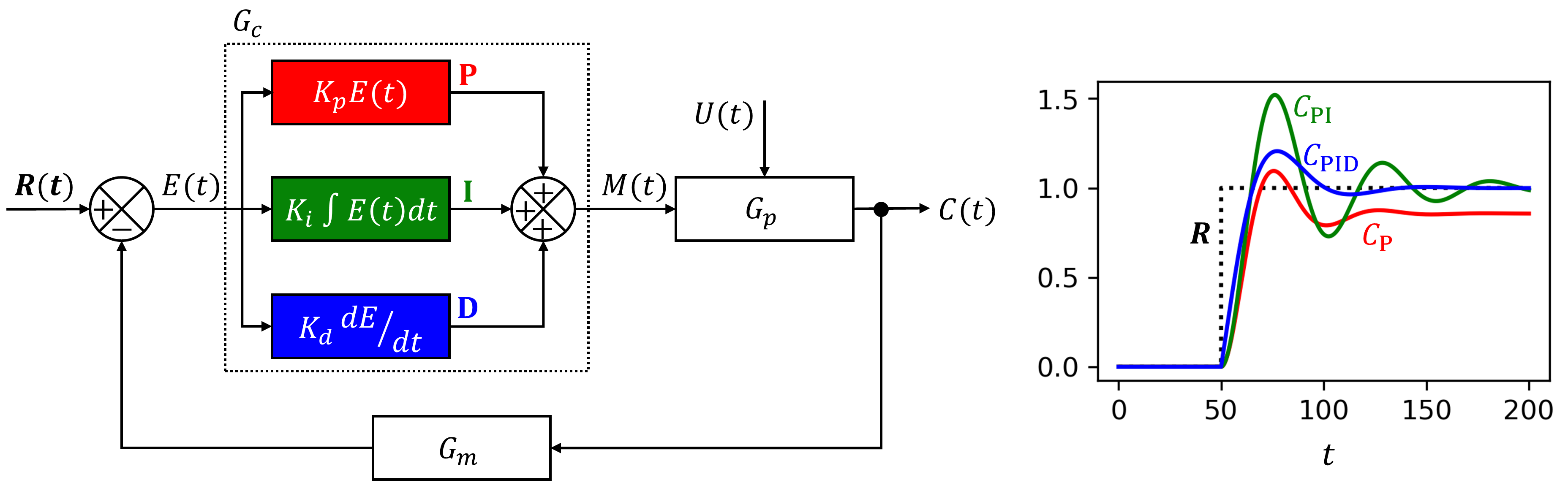
Consider a second-order plant process $G_p$. While majority of unit processes are first-order (e.g, heater, mixer, liquid tank, etc.), they are often placed in series with each other, or with measurement units $G_m$ that themselves follow first-order dynamics (though often with very small time constant). Therefore, here I consider $G_p$ as a lump of two first-order units, thereby exhibit second-order dynamics:

\begin{align} \tau^2\frac{d^2C}{dt^2} + 2\tau\zeta\frac{dC}{dt} + C(t) = M(t) + U(t) \label{eqn:ode} \end{align}

Here, $C(t)$ is the process variable, i.e., the variable we wish to control. $M(t)$ is the manipulated variable, output of the PID controller. $U(t)$ is the system load. The parameters $\tau$ and $\zeta$ control the dynamics of process $G_p$, of which real values are informed by the physical conditions of the system (e.g., heat capacitity, tank volume, flow rates, etc.).

Now onto the controller $G_c$, it takes $E(t)$ as input and yields $M(t)$ as output. $E(t)$ is the error of the process variable $C(t)$ to the setpoint $R(t)$:

\begin{align} E(t) = R(t) - C(t) \label{eqn:E} \end{align}

The controller transform $E(t)$ to $M(t)$, which then alter $C(t)$ to eventually minimize the error $E(t)$ as quickly and safely as possible. Different controller logics and parameters change how well this can be done.

The Proportional-Integral-Derivative (PID) controller is possibly the most widely used. PID controller logic works as follows:

\begin{align} M(t) = K_p E(t) + K_i \int{E(t)dt} + K_d \frac{dE}{dt} \label{eqn:M} \end{align}

The first term scales the error (P)roportionally with a factor $K_p$. The second term scales the (I)ntegral or the cumulative error with a factor $K_i$. The last term scales the (D)erivative or rate of change of the error with a factor $K_d$.

We can solve the above second-order dynamics (Eqn. \ref{eqn:ode}) by discretizing and propagating through some small timestep. While in theory regular ODE solver can deal with the second-order, it is particularly challenging because the PID logic requires knowledge of the instantaneous derivative of the $E(t)$, which makes things incredibly messy to setup (I tried).

We break the second-order ODE into two first-order ODEs. We need first a variable change,

\begin{align} c_1 &= C\\ c_2 &= \frac{dC}{dt} \end{align}

then rearangement of Eqn \ref{eqn:ode}.

\begin{align} \frac{dc_1}{dt} &= c_2 (t) \label{eqn:c1}\\ \frac{dc_2}{dt} &= \frac{1}{\tau^2}\left( -c_1(t) -2\tau\zeta c_2(t) + M(t) + U(t)\right) \label{eqn:c2} \end{align}

The practical steps—commonly known as the Euler’s numerical method—are:

Create a time array.
Create and customize arrays for time series of setpoint $R$ and load $U$ (e.g., step, pulse, wave etc.).
Initiate at $t=0$ for:
a. $c_1$ and $c_2$.
b. Error (Eqn \ref{eqn:E}), its derivative and integral, which gives $M$ (Eqn \ref{eqn:M}).
c. Initiate derivatives of $c_1$ and $c_2$ using Eqns \ref{eqn:c1} and \ref{eqn:c2}.
Iterating through each step of the predefined time array. At each step $t$:
a. Get setpoint $R$ and load $U$ at this time step from the predefined arrays.
b. Update the new $c_1$ and $c_2$ by finite difference to the previous step.
c. Update the new error components to give $M$.
d. Update the new derivatives of $c_1$ and $c_2$.

Below, we examine the PID controller in action in two scenario: 1) setpoint step-change; 2) load fluctuation.

Setpoint step-change

Here we solve the closed-loop system (controller and process) for when there is a step change in the setpoint $R$. We assume the load $U(t)$ is constant for now, and does not include in the solver. This is sometimes refered to as the “servo” problem. The Python code for solving this is shown below:

import numpy as np
##-----Process parameter-----
tau=20 #process time constant
zeta=1 #damping coefficient
##-----Controller parameter-----
Kp=2 #proportional gain
Ki=0.1 #integral gain
Kd=1 #derivative gain
##-----Time setup-----
tmax=200
dt=0.1
time=np.arange(0, tmax+dt, dt)
##-----Initial condition-----
C0=0 #intial process variable
M0=C0 #same manipulated variable as offset
##Set point and load
tstart=50
R=np.heaviside(time-tstart, 1) + C0 #Step 1 unit up from C0
U=np.zeros(len(time)) #No load considered
##-----Set up numerical solver-----
#initialize arrays
c1=np.zeros(len(time)) #C
c2=np.zeros(len(time)) #dCdt
E=np.zeros(len(time)) #E
M=np.zeros(len(time)) #M
#Initial C
c1[0]=C0 #first order
c2[0]=0 #second order
#Intial E
E[0]=R[0]-C0 #error
Ei=E[0]*dt #integral error
dE=0 #derivative error
#Initial M
M[0]=Kp*E[0] + Ki*Ei + Kd*dE + M0 #PID logic with offset
#Initial derivatives
dc1=c2[0]
dc2=1/tau**2*(-2*tau*zeta*c2[0] -c1[0] + M[0] + U[0])
##-----Solve=propagrate through time-----
for t in range(1,len(time)):
    #Update for this time step
    c1[t]=c1[t-1]+dc1*dt #first order
    c2[t]=c2[t-1]+dc2*dt #second order
    E[t]=R[t]-c1[t] #error
    Ei+=E[t]*dt #cumulate integral error
    dE=(E[t]-E[t-1])/dt #derivative error by finite difference with previous step
    #Propagate derivatives for next step
    M[t]=Kp*E[t] + Ki*Ei + Kd*dE + M0 #PID logic with offset
    dc1=c2[t]
    dc2=1/tau**2*(-2*tau*zeta*c2[t] -c1[t] + M[t] + U[t]) 
##-----Plot-----
import matplotlib.pyplot as plt
plt.plot(time, R) #setpoint
plt.plot(time, c1) #process varibable
plt.plot(time, M) #manipulated variable
plt.plot(time, E) #error
plt.show()

\[K_p\] 0

\[K_i\] 0

\[K_d\] 0

As you play with the above interactive plot, consider these aspects:

Manually tune the PID parameters

There are numerical methods to optimize these parameters to meet various criteria (e.g., quarter-wave decay). Here let’s just try a simple manual tuning exercise:

From an initial system with all $K$’s equal 0, move only $K_p$ up until the process variable ($C$) oscillate with a small overshoot (i.e., going above the setpoint $R$).
Here we see the steady-state (i.e., the long-time plateau) of $C$ does not quite match $R$, which is known problem with using just the (P)roportional controller. Increase $K_i$ very slightly until we see steady-state $C$ matches well with $R$.
Now we perhaps want to reduce the time it takes to reach steady-state or reduce the overshoot. Increase $K_d$ to do just that.

Observe controller instability

Controller’s stability is an important consideration. To visualize how instability manifests, with a small $K_p$, keep increasing $K_i$ until the oscillation starts to progressively increase with time and never reaches the $R$ target.
Intuitively, this is because the (I)ntegral error component penalizes the cumulative deviation of $C$ to $R$. Therefore, at some critical $K_i$ weight, more cumulative error leads to more corrective action that overshoots the target, leading to even more culmulative error, and so on.

Observe spike in manipulated variable

While a controller’s objective is to match process variable $C$ to setpoint $R$, how the manipulated variable $M$ manifests is also important. To demonstrate, at some small $K_p$ and $K_i$, increase $K_d$ to the max level. We see while increasing the (D)erivative error helps to “smooth” out the process variable dynamics, there is a conspicuous spike in the manipulated variable $M$. This is because the (D) component penalizes sudden changes in the error, thereby aggressively responses to a step-change in setpoint. In physical systems, manipulated variables $M$ usually transfer to gas pressure for pneumatic valves, of which spikes could be a safety hazard or downright un-actuatable (that’s a word?) by the equipment.

Load fluctuation

Here we consider a constant setpoint $R$ but with changing and fluctuating load $U$. This is refered to as a “regulator” problem, which is perhaps more common for chemical engineers.

To set this problem up, we simply re-customize our setpoint $R$ and $U$ functions. To simulate noise or fluctuation of the load change, we can sample from a normal distribution with preset average $\Delta U$ ($\Delta$ because it is a change from previous value), and standard deviation $\delta U$.

##Set point and load
#Setpoint held constant at 1
R=np.zeros(len(time))+1
#Load fluctuation
tstart=200 #time when load changes
delU=10 #how much load change
stdU=2 #how much new load fluctuate
U=np.zeros(len(time))
for i in range(len(U)):
    #Randomize load with a normal distribution
    if time[i] <= tstart: U[i]=np.random.normal(loc=0, scale=1)
    else: U[i]=np.random.normal(loc=delU, scale=stdU)

\[\Delta U\] 0

\[\delta U\] 1

\[K_p\] 0

\[K_i\] 0

\[K_d\] 0

From above interactive plot, we can see how the fluctuation in load $U$ manifest into the process variable $C$. The controller effectively dampens the fluctuation such that the fluctuation of $C$ is stretched out over a longer time period in comparison to that of $U$. As of now, I am not sure whether the PID $K$’s parameters affect the damping of $C$’s fluctuations.